How to compare two lists or sheets in Excel and find the differences
Spreadsheet tools · Published
Find what's in one list but not the other, spot matching and changed rows, and highlight differences between two sheets, with formulas that work in every Excel version.
The short answer
To find items in one list that are missing from another, add a helper column with COUNTIF. It counts how often each item appears in the other list, so 0 means "missing". It works in every version of Excel.
To compare two sheets that have the same layout, compare them cell by cell with a formula such as =B2<>Old!B2, then highlight the differences with conditional formatting. The sections below cover both, plus the spaces and capital letters that make identical-looking values fail to match.
Find items missing from the other list
Say column A holds this month's customer IDs and column B holds last month's. You want to know who is new and who has dropped off.
- In C2, type the formula below and press Enter.
- Double-click the fill handle (the small square at the cell's bottom-right corner) to copy it down to the end of list A.
- Filter or sort column C to see every "No" together: those IDs are only in list A.
=IF(COUNTIF($B$2:$B$6,A2)>0,"Yes","No")COUNTIF($B$2:$B$6,A2) counts how often the value in A2 appears in last month's list. The dollar signs lock that range so it doesn't move when you copy the formula down, while A2 changes to A3, A4 and so on. IF then turns any count above zero into "Yes" and zero into "No". Change the range to cover your whole list, for example $B$2:$B$500.
Check the other direction with MATCH
To find last month's customers who aren't in this month's list, swap the lists. This version uses MATCH:
=IF(ISNUMBER(MATCH(B2,$A$2:$A$6,0)),"Found","Missing")MATCH looks for B2 in list A. The 0 at the end asks for an exact match. If it finds the value, it returns its position (a number); if not, it returns #N/A. ISNUMBER turns that into TRUE or FALSE, and IF writes the label.
| Row | A | B | C | D |
|---|---|---|---|---|
| 1 | This month | Last month | In last month? | Still a customer? |
| 2 | C-101 | C-104 | Yes | Found |
| 3 | C-102 | C-101 | Yes | Found |
| 4 | C-103 | C-107 | No | Missing |
| 5 | C-104 | C-102 | Yes | Found |
| 6 | C-105 | C-108 | No | Missing |
So C-103 and C-105 are new this month, and C-107 and C-108 didn't come back.
With XLOOKUP (Microsoft 365, Excel 2021 and later)
If you have XLOOKUP, this formula returns the matching ID, or the text you choose when there's no match:
=XLOOKUP(A2,$B$2:$B$6,$B$2:$B$6,"Not in last month")The arguments are: what to find (A2), where to look (list B), what to return (list B again), and what to show if it isn't there. Microsoft says XLOOKUP isn't available in Excel 2016 or Excel 2019; there you'll see #NAME?, so use COUNTIF instead. For more on the lookup functions, see VLOOKUP vs XLOOKUP vs INDEX/MATCH.
Highlight the missing items with conditional formatting
If you'd rather color the cells than add a column:
- Select A2:A6 (the first list, without its header).
- Go to Home › Conditional Formatting › New Rule. On a Mac, set Style to Classic first.
- Choose Use a formula to determine which cells to format.
- Enter the formula below.
- Select Format (Format with › Custom Format on a Mac), pick a fill color and select OK.
=COUNTIF($B$2:$B$6,$A2)=0Write the formula for the first selected cell (A2). Excel adjusts it for the other cells, so C-103 and C-105 turn colored. Excel for the web also has conditional formatting, but its screens differ from the steps above.
Compare two sheets row by row
When two sheets have the same rows in the same order (an old and a new price list, say), you can compare them cell by cell. Here the sheets are named Old and New.
- On the New sheet, add a column next to the data.
- In C2, enter the formula below and copy it down.
Old!B2means "cell B2 on the sheet called Old". - To check names including capital letters, add
=EXACT(A2,Old!A2)in D2. The normal=comparison ignores case; EXACT doesn't.
=IF(B2<>Old!B2,"Changed","Same")| Row | A | B |
|---|---|---|
| 1 | Product | Price |
| 2 | Desk lamp | 24.99 |
| 3 | Chair | 89 |
| 4 | Shelf | 45.5 |
| 5 | Rug | 60 |
| Row | A | B | C | D |
|---|---|---|---|---|
| 1 | Product | Price | Price changed? | Same name? |
| 2 | Desk lamp | 24.99 | Same | TRUE |
| 3 | Chair | 94 | Changed | TRUE |
| 4 | Shelf | 45.5 | Same | TRUE |
| 5 | rug | 55 | Changed | FALSE |
To color the changed prices instead, select B2:B5 on New and create a formula rule as above with =$B2<>Old!$B2. Conditional formatting can refer to another sheet in the same workbook, but Microsoft says it can't use references to another workbook. If your sheets are in two files, copy one sheet into the other workbook first.
Why identical values don't match
- Extra spaces. "C-101 " with a trailing space isn't the same as "C-101", so COUNTIF returns 0. Wrap the value in TRIM:
=COUNTIF($B$2:$B$6,TRIM(A2)), or clean both lists first with the steps in how to clean up text in Excel. - Capital letters. COUNTIF and MATCH ignore case, so "c-101" matches "C-101". Use EXACT when case matters.
- Numbers stored as text. An ID typed as text (often shown with a small green triangle) may not match the same number in the other list. Convert one list so both are the same type.
- Wildcards. COUNTIF treats
*and?in the value as wildcards, so a code containing them can match more than you expect. MATCH with 0 has the same behavior for text.
If one list has repeated entries, see how to find duplicates in Excel before comparing.
Other ways to compare
Microsoft's Spreadsheet Compare, a separate Windows app, compares two whole workbooks and lists every changed cell. Microsoft says it's only included with Office Professional Plus 2013, 2016 and 2019 and with Microsoft 365 Apps for enterprise, so many home and business plans don't have it.
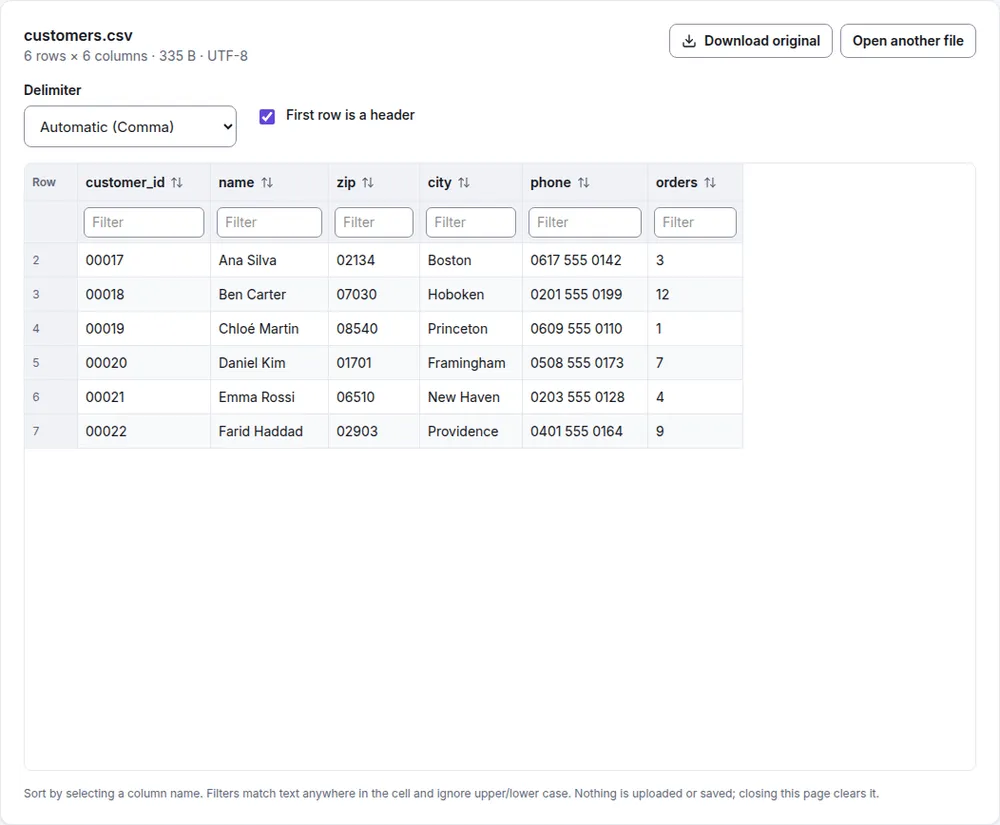
If your lists come from two exports as CSV files, you can look through them before opening Excel. Filecon's CSV viewer opens a CSV in your browser without uploading it. Sort a column or type an ID into a column filter to check whether it's there, and values are shown exactly as written in the file, spaces and leading zeros included.
In short
Use COUNTIF (or MATCH, or XLOOKUP in newer Excel) with an ID to find items that are only in one list, and check both directions. Compare sheets cell by cell only when their rows line up, and use a conditional formatting rule to make the differences stand out. When a match fails for no visible reason, look for spaces, text-versus-number cells and capital letters.